A Modeling Approach
Philosophy of Science
I define reality as consisting of all that exists. This includes not only what we typically think of as physical stuff – like trees, houses, cars, and people – but also things like ideas, beliefs, feelings, etc. You might consider me a physical monist, in that I do not make distinctions between physical and “non-physical” objects. I think if things like ideas as emergent properties of our brains functioning within many layers of context. This belief has a few implications worth noting. First, it assumes that we all live in the same reality – what I do can have an impact on you and what you do can impact me.
However, I am convinced that this reality is extremely complicated. In fact, I am skeptical that we can ever fully understand reality (and by we I mean as a species, much less as individuals).
Does this mean we cannot understand reality at all? I don’t think so. I don’t fully understand how my car works, but I do have basic ideas that allow me to problem solve issues such as when it won’t start. When we can’t fully understand something, we are left to build an model of that process. I will talk more about models below, but for now think of a model as an oversimplified representation of a much more complex system. We all create models of reality, and the models we create depend on our values, knowledge, experiences, context, and goals, to name only a few.
So, as I see it, modeling is not an option, we all must do it. Furthermore, the oversimplification of reality is not a limitation of science, but is necessary for its progress.
The Modeling Approach
A great introduction to the modeling approach is an article by Rodgers (2010). I highly recommend reading this article, as it give a great overview of the limitations of strict hypothesis testing, and the advantages of using a modeling approach.
What are Scientific Models?
Models are explicit statements about the processes that give rise to observed data. - Little (2013)
A mathematical model is a set of assumptions together with implications drawn from them by mathematical reasoning. - Neimark and Estes (1967 quoted in Rodgers, 2010)
Goals of science
Often, the three goals of science are stated:
- Describe
- Predict
- Explain
Models are important for all these goals.
Models are representations of how our key constructs are related. They can be narrative, graphical, or mathematical. Models match reality in some way, and are simpler than reality.
Why do we need models?
If we acknowledge the .red[complexity] and .red[interrelatedness] of reality, and our goal is the perfect model, we soon realize To model anything, we would have to model everything!
All models are wrong, but some are useful -George Box
Occam’s Razor
- We need to balance explanatory power (reducing error) with parsimony (simplicity)
- We want to constantly ask: “What do we gain by adding complexity?”
- Proportion Reduction in Error (PRE)
Scientific Models are NOT Oracles

Scientific Models are Golems

Simple Models: Errors and Parameters
The Basic Model
Narrative, Numeric, and Graphical Models
Let’s start with a simple narrative model:
“Peer pressure causes smoking.”
We can start to convert this to other forms of model. It is often helpful to take our narrative model an turn it into a graphical model.
Here is a simple graphical model of our example model:
Here is a generalized graphical representation of our model.
Here is the general form of a numerical model (an equation) with the three main components: \[ \text{DATA} = \text{MODEL} + \text{ERROR} \] where,
- DATA = What we want to understand or explain
- MODEL = A simpler representation of the DATA
- ERROR = Amount by which the model fails to explain the data
What is another term for error?
We could take our graphical model and turn it into an equation:
\[ \text{Smoking} = \text{Friend Smokes} + \text{ERROR} \]
A Simple Model
A mathematical representation
\[ \text{DATA} = \text{MODEL} + \text{ERROR} \] Population model:
\[ Y_i = \beta_0 + \varepsilon_i \]
Sample model:
\[ y_i = b_0 + e_i \]
Describing Error
Simplest Model
Zero Parameters
\[ Y_i = B_0 + \varepsilon_i \]
Where \(B_0\) is some a priori value, not based on these DATA, but provided by some theoretical consideration
- e.g. temperature = 98.6 degrees
- probability if coin is fair = .50
- change over time = 0
Not common in behavioral sciences
Simple Model
One Parameter
\[ Y_i = \beta_0 + \varepsilon_i \] Where \(\beta_0\) is an unknown value. The MODEL makes a constant prediction for all cases, but the value of that prediction is to be estimated from the data, so to make ERROR as small as possible.
The estimated MODEL is
\[ Y_i = b_0 + e_i \]
Where \(b_0\) is the actual prediction made for each case, estimated from the data, minimizing ERROR.
This estimated MODEL can also be written as
\[ \hat{Y_i} = b_0 \]
Note the difference between the two errors in the parameter model ( \(\varepsilon_i\) ) and the estimated model ( \(e_i\) ). The latter is an estimate of the former, just as \(b_0\) is an estimate of \(\beta_0\).
\[ \varepsilon_i = Y_i - \beta_0 \]
\[ e_i = Y_i - b_0 = Y_i - \hat{Y_i} \]
Measures of Central Tendency and Dispersion
- Want to find best estimate of \(\beta_0\) that minimizes not individual \(e_i\)’s but some aggregate measure of error.
- Different ways of aggregating errors lead to different estimates - alternative measures of Central Tendency
- Different ways of aggregating errors lead to different estimates of “Typical Error” - alternative measures of Spread
- This is “descriptive statistics”
Measures of Central Tendency and Dispersion
Minimize Sum of Errors? - Why not?
Minimize Sum of Absolute Errors (SAE). - best estimate of \(\beta_0\) is the Median
What happens in presence of extreme outlier?
Absolute Errors and Outliers
Median Absolute Deviation (MAD) as typical measure of spread (median value of \(e_i\) given minimization of SAE)
Measures of Central Tendency and Dispersion
- Minimize Sum of Squared Errors. Why?
- best estimate of \(\beta_0\) is the Mean
- What happens in presence of outlier?
- Squared Errors and Outliers -Mean Square Error (Variance) as typical measure of spread (mean value of \(e_i^2\) given minimization of SSE)
Formalities of Estimation
Simple Model
DATA = MODEL + ERROR
\[ Y_i = \beta_0 + \varepsilon_i \] \[ Y_i = b_0 + e_i \] \[ \hat{Y_i} = b_0 \] \[ Y_i = \hat{Y_i} + e_i \]
\[ e_i = Y_i - \hat{Y_i} \]
Aggregate Error: Sum of Absolute Errors
\[\text{Error} = \sum_{i=1}^{n} |e_i| = \sum_{i=1}^{n}|Y_i - \hat{Y_i} | = \sum_{i=1}^{n} | Y_i - b_0|\]
- Minimization estimates \(\beta_0\) as the Median
- Measure of Spread: Median Absolute Error or Median Absolute Deviation (MAD)
Aggregate Error: Sum of Squared Errors
\[\text{Error} = \sum_{i=1}^{n} e_i^2 = \sum_{i=1}^{n} (Y_i - \hat{Y_i})^2 = \sum_{i=1}^{n} (Y_i - b_0)^2 = \sum_{i=1}^{n} (Y_i - \bar{Y})^2\]
- Minimization estimates \(\beta_0\) as the Mean
- Measure of Spread: Mean Squared Error (Variance)
Mean Squared Error Estimation
- Recall that if one estimated \(n\) parameters, ERROR would be zero.
- In computation of the MSE, we want to take into account the number of parameters estimated (and the number of additional parameters that could be estimated).
- General formula for MSE:
\[\text{MSE} = \frac{ \sum_{i=1}^{n} (Y_i - \hat{Y_i})^2}{n-p}\]
- Square root known as the “root mean square error”
Mean Squared Error Estimation
- In case of simple one-parameter model, \(p = 1\) and
\[\hat{Y_i} = b_0 = \bar{Y}\]
Accordingly,
\[\text{MSE} = \frac{ \sum_{i=1}^{n} (Y_i - \hat{Y_i})^2}{n-1} = s^2\]
And root mean square error is called the standard deviation
So variance is special case of MSE; MSE as unbiased measure of spread (or variance) of errors
Usual notion: descriptive statistics
Pick a measure of central tendency (mean, median, mode)
Pick a measure of spread
NO - pick a measure of aggregate error, estimates of \(\beta_0\) follow from that, along with estimates of typical error.
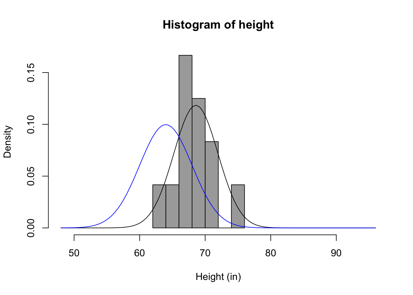
An Example
       vars  n  mean   sd median trimmed  mad  min max range skew kurtosis   se
repht     1 12 67.83 3.66  68.00   67.80 2.97 61.0  75  14.0 0.10    -0.51 1.06
height    2 12 68.58 3.37  68.25   68.55 2.59 62.5  75  12.5 0.13    -0.72 0.97
repht height
repht 1.0000000 0.9804921
height 0.9804921 1.0000000Distribution of measured heights

